
Clustering riders
Today we address a complex, but fun and interesting problem: clustering riders. This is by far a new idea, everybody knows Elia Viviani and Dylan Groenewegen are classified as ‘sprinters’, whereas Chris and Froome are ‘GC guys’. The label a rider receives is simply based on past results. We are going to investigate whether we can take this a step further by (1) using a uniform point system for race results and (2) including other dimensions than just outcomes. One of our findings is that although Dylan Groenewegen and Elia Viviani are both sprinters, they clearly belong to different clusters. Let’s dive in and investigate how we came to this conclusion.
Truth to be told, clustering is an art as well as a science. It is a very exploratory type of analysis where you try to find subgroups of observations (in our case riders) that are most similar across the dimensions that you consider. Clustering requires substantial thought about the algorithm to use, the outcomes you include and whether you scale them in a particular manner. The results are in general not right or wrong, but should help you gain insights in a particular field.
In our rider cluster procedure we consider the following 11 dimensions:
- ODR flat Points scored in flat one day races
- ODR not-flat Points scored in one day races that are not flat
- ODR unknown Points scored in one day races for which we could not determine the profile
- TT Points scored in time trials during a race
- stage MT Points scored in mountain stages
- stage flat Points scored in flat stages
- stage hill Points scored in hilly stages
- stage hill-flat Points scored in hilly stages, but with a reasonably flat finish
- GC Points scored in GC’s (excluding youth/mountain/points/combat classifications)
- % WT Percentage of points scored at the UWT level
- % May Percentage of points scored before May 1
All variables are calculated for the riders that are part of the 2019 World Tour teams. We require that a rider scores at least 50 points and participates in at least 20 single day races or race stages before we include him in the analysis.
Nine out of 11 variables use ‘points’. We do not use UCI points or rank scores for the analysis. Instead, we use a point system very similar to the Zweeler games, where finishing first in a race stage yields 35 points. For a one day race a rider can earn up to 120 points. With this point system it pays off to finish in the top 20 (stage) or top 25 (one day race). It is good to know that we rescale the points variables per rider. For example, ‘TT’ is the percentage of the total rider points scored in time trials.
The GC points are calculated as the number of stage points times the square root of the race length. As a consequence a grand tour victory yields the same amount of points as about 4.5 stage wins. The points may not be perfectly balanced, but keep in mind the main purpose of the points is to determine the strengths of riders, we will not really use them to claim one rider is ‘better’ than another.
Unlike UCI points the Zweeler points to not change by race class (World Tour, HC, etc). We really do this on purpose, it allows us to identify riders that are similar to e.g. Peter Sagan or Greg van Avermaet in their race preferences and performance, but don’t show this at World Tour level. This could be because of their race preferences, perhaps they simply cannot compete with the absolute top or have team orders that prevent them from riding for their own chances. To compensate for the level the results were obtained on we have ‘% WT’ which is the percentage of points scored at the World Tour level. With the variable ‘% May’ (the percentage of points scored before May 1st) we try to capture the form peak of riders.
Now before we can show some results we are left with one big question. How many groups of riders are there? Fortunately, this is not a trial and error process. There are several techniques that can be used to determine the number of clusters. One of these approaches is the ‘silhouette’ method and the results are shown in Figure 1. The method indicates the optimal number of groups is 9, however, the difference with 7 or 8 clusters is small. For now we stick with 9 clusters and let’s see what comes out.
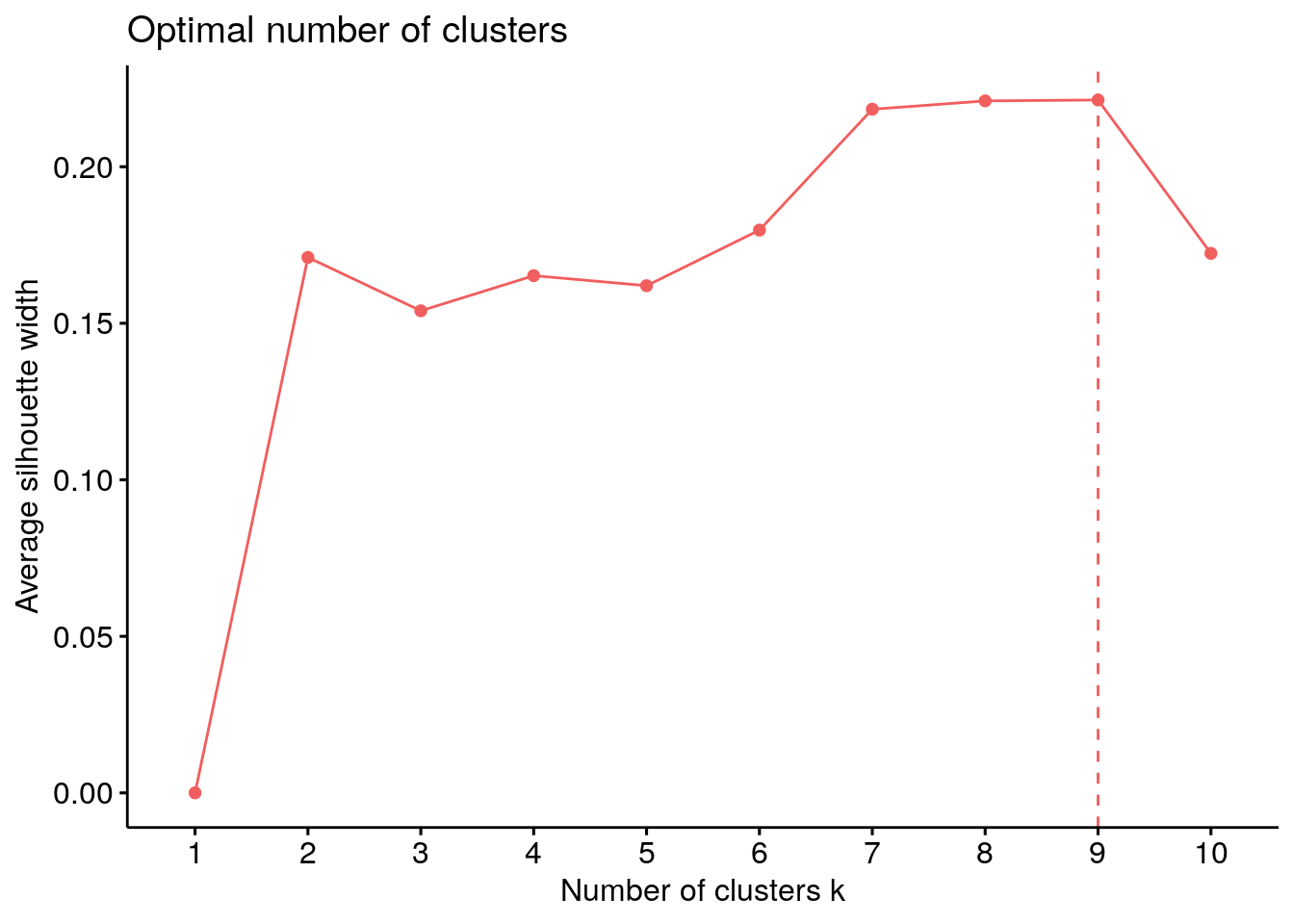
Figure 1: Optimal number of clusters using silhouette appraoch.
Just to recap, we have 11 variables / dimensions and the algorithm indicates we should make 9 groups / clusters of riders with those variables. The resulting clusters are presented in two different ways. Figure 2 shows the scores of each cluster in a radial plot. It is quite intuitive to read and observe the differences between clusters. For example, lets focus on the grey-blue line (cluster number 1). The riders in this cluster score very high in the variables % WT and % May and take most those points from not flat single day races (ODR not-flat). Compare this with cluster 9. These riders also score high on the not flat single day races, but do this in general after May and not so much on a world tour level.
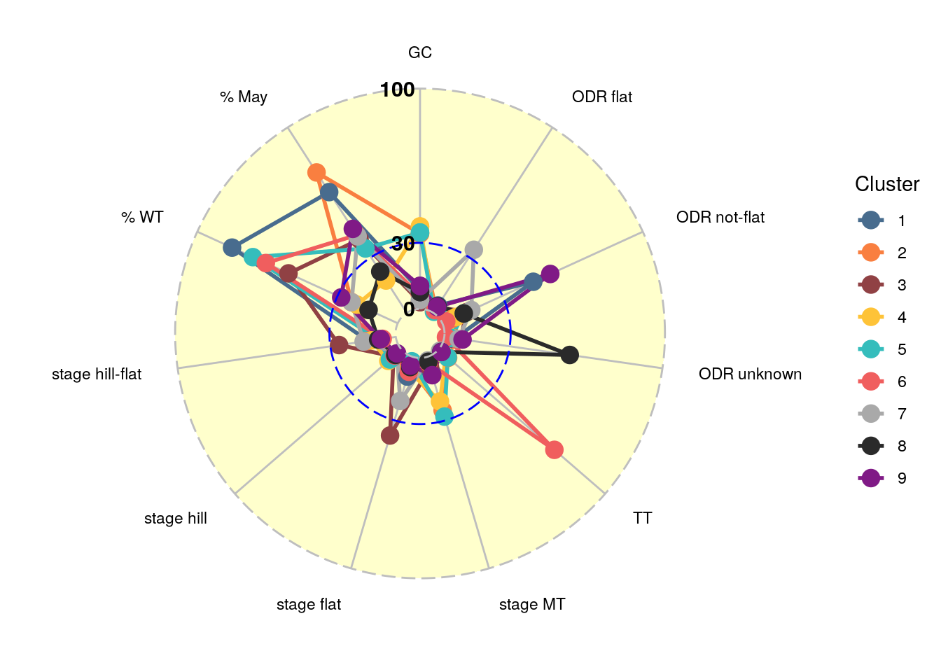
Figure 2: Scores per dimension for each cluster in a radial plot.
Some big names from cluster 1 are Greg van Avermaet and Peter Sagan, but guess who is in cluster 9: Alejandro Valverde . Well, yeah that can happen, if you let a computer do the job, but let’s just take a quick peek whether this makes sense given the variables. Figure 3 shows the scores for the most characteristic riders for cluster 1 (Daryl Impey) and cluster 9 (David Gaudu) as well as Peter Sagan (cluster 1) and Alejandro Valverde (cluster 9). The difference between the two groups can be explained by, among others, the percentage of points at World Tour level and points scored in hilly stages. Furthermore, Valverde and Gaudu tend to score more in GC’s. At some point we will also consider more advanced cluster types where each rider can actually be part of multiple clusters. It is likely that members of cluster 1 are also to some extent part of cluster 9 and vice versa.
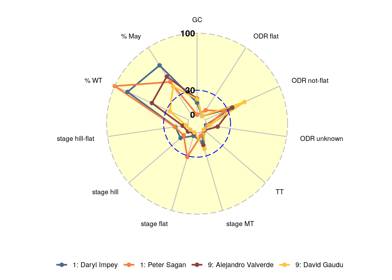
Figure 3: Scores per dimension for D. Impey and P. Sagan (cluster 1) / A. Valverde and D. Gaudu (cluster 9)
If you are completely confused by these ‘spider webs’, take a look at a different representation of the clusters in Figure 4. The figure contains the scores of each cluster in a single bar. Each bar has colors that correspond to the variables and larger/smaller chunks indicate that the members of that cluster score in general high/low on that outcome measure. With these bars we made an attempt to characterize each cluster in a few words. These short descriptions are shown in Table 1. In this table you can also find the 5 most characteristic riders in each cluster. The characteristic riders should be exemplary for the cluster. Furthermore, the table also contains the riders that scored most points in each cluster. Please remember, this does not necessarily mean that these are the best riders in the cluster.
Figure 4: Scores per dimension for each cluster in a stacked bar chart.
Since this is already quite a lengthy post let’s check out the sprint clusters 3 and 7 characterized by Giacomo Nizzolo and Fabio Jakobsen, respectively. The radial/spider plots of these clusters are shown in Figure 5 and Figure 6. The differences between the two clusters are actually quite obvious. Cluster 3 contains sprinters that are really focused on the flat race stages, and get most of their points from World Tour races. The sprinters in cluster 7 still do very well on the flat stages (look at the points relative to the dashed blue circle), but score quite some points in one day races.
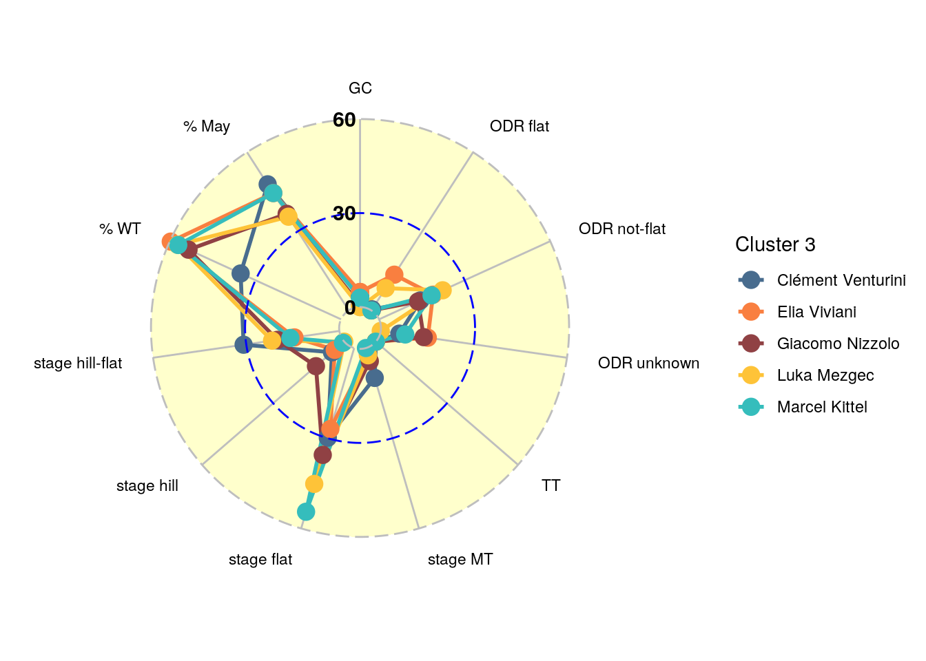
Figure 5: Scores per dimension for sprint cluster 3.
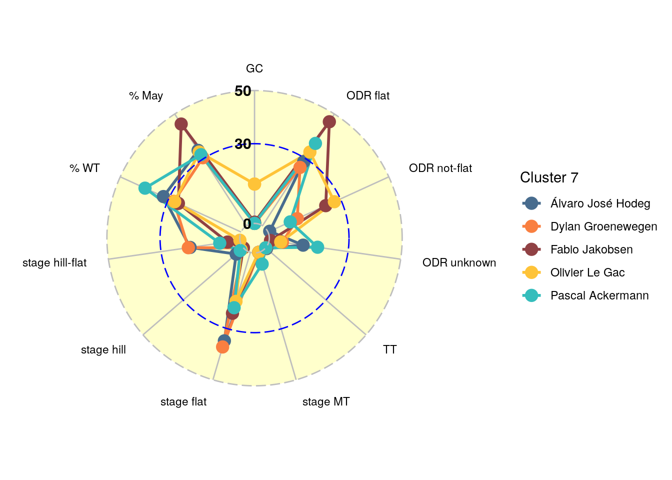
Figure 6: Scores per dimension for sprint cluster 7.
Hopefully you enjoyed the insights. We are aware that there is plenty of room for improvement. In the future we will look more into the variables included in the analysis and we will also investigate whether it is insightful to allow for multiple cluster memberships. If you have any other suggestions, or if you would like to see some more figures of different clusters let us know on Twitter or by mail.
Update 2019-03-22: we will try to update the results in this post in the beginning of March. In this update we will try an alternative ‘two-step’ approach, where we leave out the variables %WT and %May in the first step. This will most likely lead to a more traditional result (less cluster) of e.g. sprinters, GC guys, ODR specialist and time trialists. Subsequently we will use more detailed features to create clusters within each group to identify e.g. different types of sprinters.