Clustering riders: an improved approach

The old and new approach

In our first attempt we used the following dimensions to cluster riders in a single step:

• ODR flat Points scored in flat one day races
• ODR not-flat Points scored in one day races that are not flat
• ODR unknown Points scored in one day races for which we could not determine the profile
• TT Points scored in time trials during a race
• stage MT Points scored in mountain stages
• stage flat Points scored in flat stages
• stage hill Points scored in hilly stages
• stage hill-flat Points scored in hilly stages, but with a reasonably flat finish
• GC Points scored in GC’s (excluding youth/mountain/points/combat classifications)
• % WT Percentage of points scored at the UWT level
• % May Percentage of points scored before May 1

The result was 9 different clusters, but many clusters were quite alike and there were e.g. 3 clusters that were GC related, but the distinction came from the ‘% WT’ and ‘% May’ variables. These variables do not really characterize the type of rider but the level and moments of peak performance. Hence, it is more natural to look at these when they main groups are already determined. Furthermore, there is also a risk that riders from a different group (e.g. a sprinter) is put in a GC group because of great similarity in ‘% WT’ and ‘% May’.

In this post we will take a different approach and do the following:

1. We are going to make initial clusters on less dimensions. This most likely leads to fewer clusters that are clearly defined as GC, sprinter, etc. The eight dimensions that remain from the first version are: GC, ODR flat, ODR non-flat, TT, stage MT, stage flat, stage hill, and stage hill-flat. We introduce one new dimension: points from mountain classifications. Due to the fact that we count points for flat stages and hilly stages with a flat finish we do not award points for being in the final point classification. The total number of dimensions in the first step is nine.
2. We stop using Zweeler points. Instead, we use a different point calculation where each top 20 classification yields points, with the number one earning 20 points and the number 20 gets 1 points. Riders get points for race stages, GC’s, MC’s (mountain classifications), and one day races. The GC / MC points are adjusted for race length, such that grand tours matter most. The 1.UWT classics points get a multiplier of 1.5.
3. The points are re-scaled per rider as we are interested in the source of the points, not necessarily the number of points. This is unchanged compared to our first clustering post.
4. Once we have obtained initial clusters, we are going to cluster again within each cluster to discover the different types of e.g. sprinters. In the second stage clustering procedure we will use additional variables such as ‘% WT’ and ‘% May’. An advantage of this approach is that we can change the second stage variables, dependent on the cluster that we investigate. For example, we will take a closer look at the sprinter cluster and use variables related to average race length and race speed.

The first step clustering results are outlined in the next section.

Step 1: general clusters

Figure 1 shows that, with our nine dimensions, the optimal number of clusters in the first step is four. The radial plot that shows the scores on each dimension for the four clusters is provided in Figure 2.

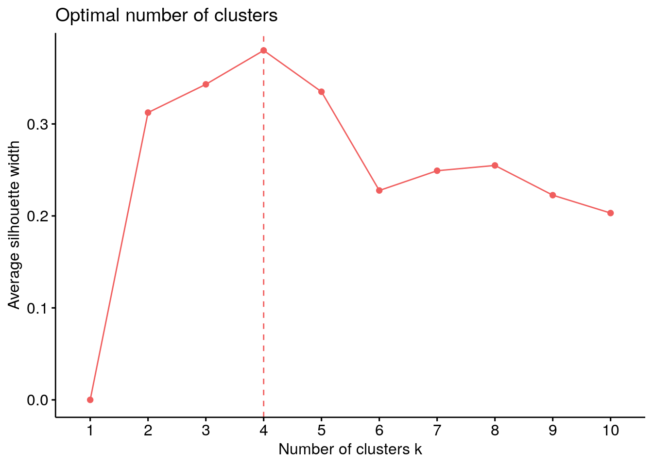
Figure 1: Optimal number of clusters using silhouette appraoch.

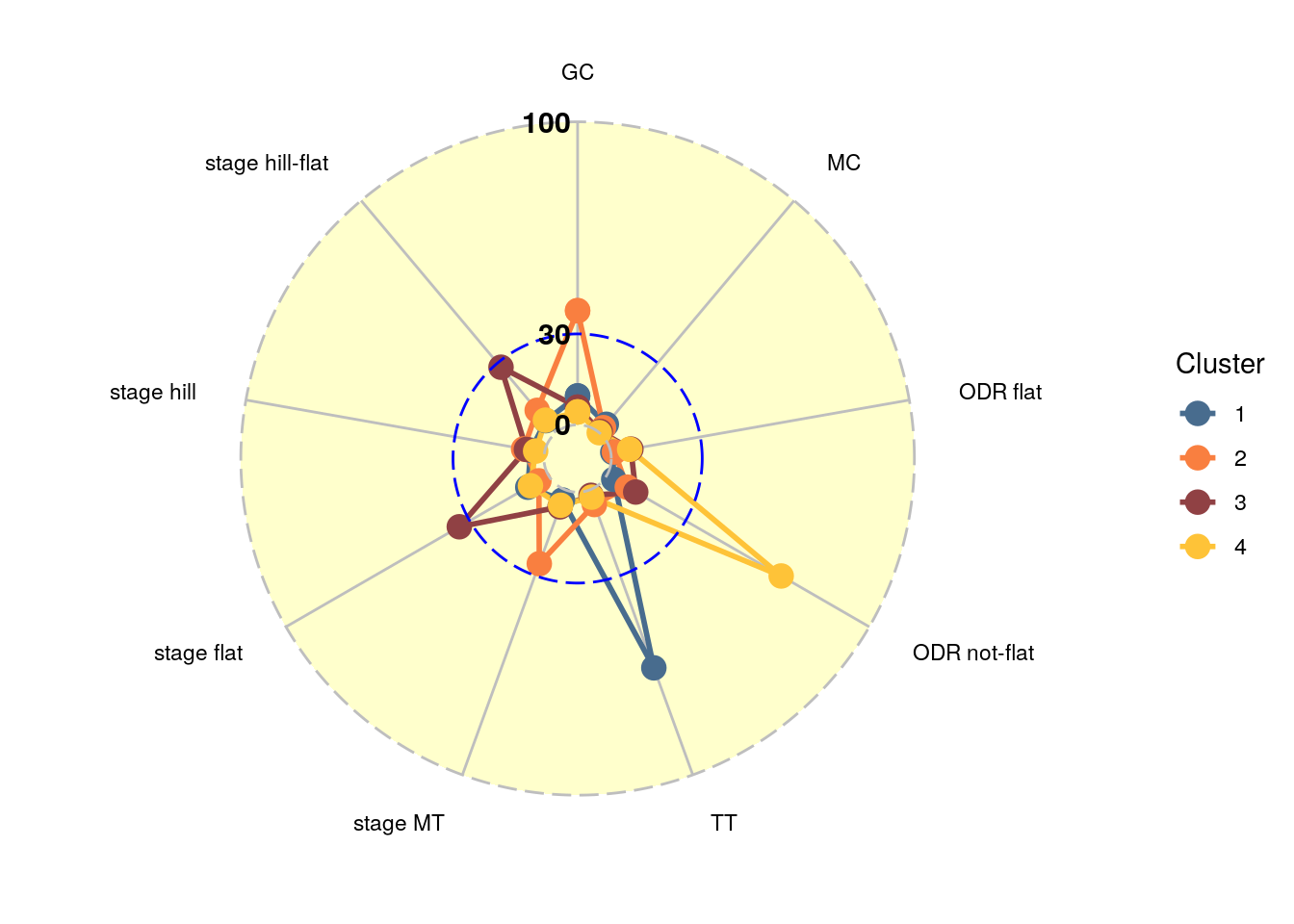
Figure 2: Scores per dimension for each cluster in the first step in a radial plot.

From Figure 2 it quickly becomes clear that especially the classic specialists (cluster 4) and time trialists (cluster 1) gain their points from mainly one dimension. The sprinters in cluster 3 get their points from the different types of flat finishes, whereas the riders in cluster 2 score in mountain stages and GC’s. A bar chart representation of the scores on each dimension is provided in Figure 3.

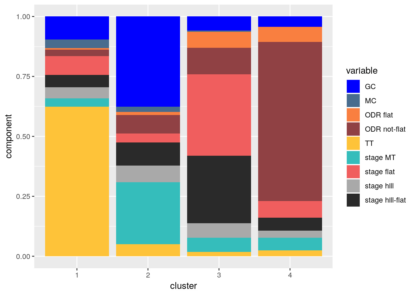
Figure 3: Scores per dimension for each cluster in the first step but now in a stacked bar chart.

The four cluster outcomes are very logical and in fact these are the four categories on the PCS profiles (e.g. Alejandro Valverde)! It is a confirmation that the clustering method is sensible. In addition, it also shows that the profile scores on PCS are well thought of 😀 Before we will zoom in on the sprint cluster, we have outlined for each initial cluster the most characteristic riders (most exemplary) of each cluster as well as the riders with most points in each cluster.

cluster 4: classics specialists (26 riders)

• most characteristic: Oliver Naesen, Robert Power, Sep Vanmarcke, Łukasz Wiśniowski, Michael Valgren
• top scoring: Oliver Naesen, Robert Power, Sep Vanmarcke, Łukasz Wiśniowski, Michael Valgren

To illustrate the concept of ‘most characteristic’ rider a bit more, take a look at Figure 4. Here you can see the scores on each dimension of the most characteristic sprinters in cluster 3. As you can see these riders indeed have quite a similar profile across all variables we consider in step 1. In the next section we will dive further into this sprint cluster and introduce new variables that allow us to split up this group further.

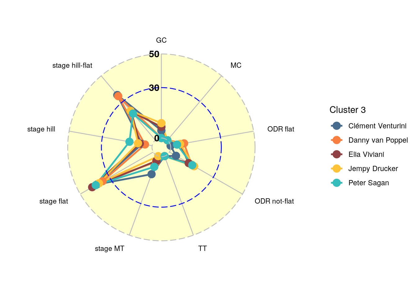
Figure 4: Scores per dimension for first step sprint cluster 3.

Step 2: re-clustering sprint cluster 3

For the second step we are going to focus on the 97 sprinters in cluster 3. We will cluster these sprinters again and use the following additional variables:

• % WT Percentage of points scored at the UWT level
• % May Percentage of points scored before May 1
• team pos The average relative position of the rider within the team
• % high speed Percentage of points scored in the 25% of races with the highest average speed
• % 200+ km Percentage of points scored in races/stages with more than 200 kilometers

The additional variables should be reasonably self-explanatory, except for the ‘team pos’ variable. We introduce this variable to account for the fact that a lead-out may very well end up in the top 20 as well, but most likely behind the protected rider. Since we do not use the total number of points scored in the clustering we do look at how high ranked is a rider within his team. So for each race we look at the rank of a rider within his own team, re-scale this on the 0-100 domain and average it over all races the rider participates in.

With the additional five variables (now 14 in total) the optimal number of clusters for the 97 sprinters is three (Figure 5) and the scores of the three clusters on each of the 14 dimensions can be found in Figure 6.

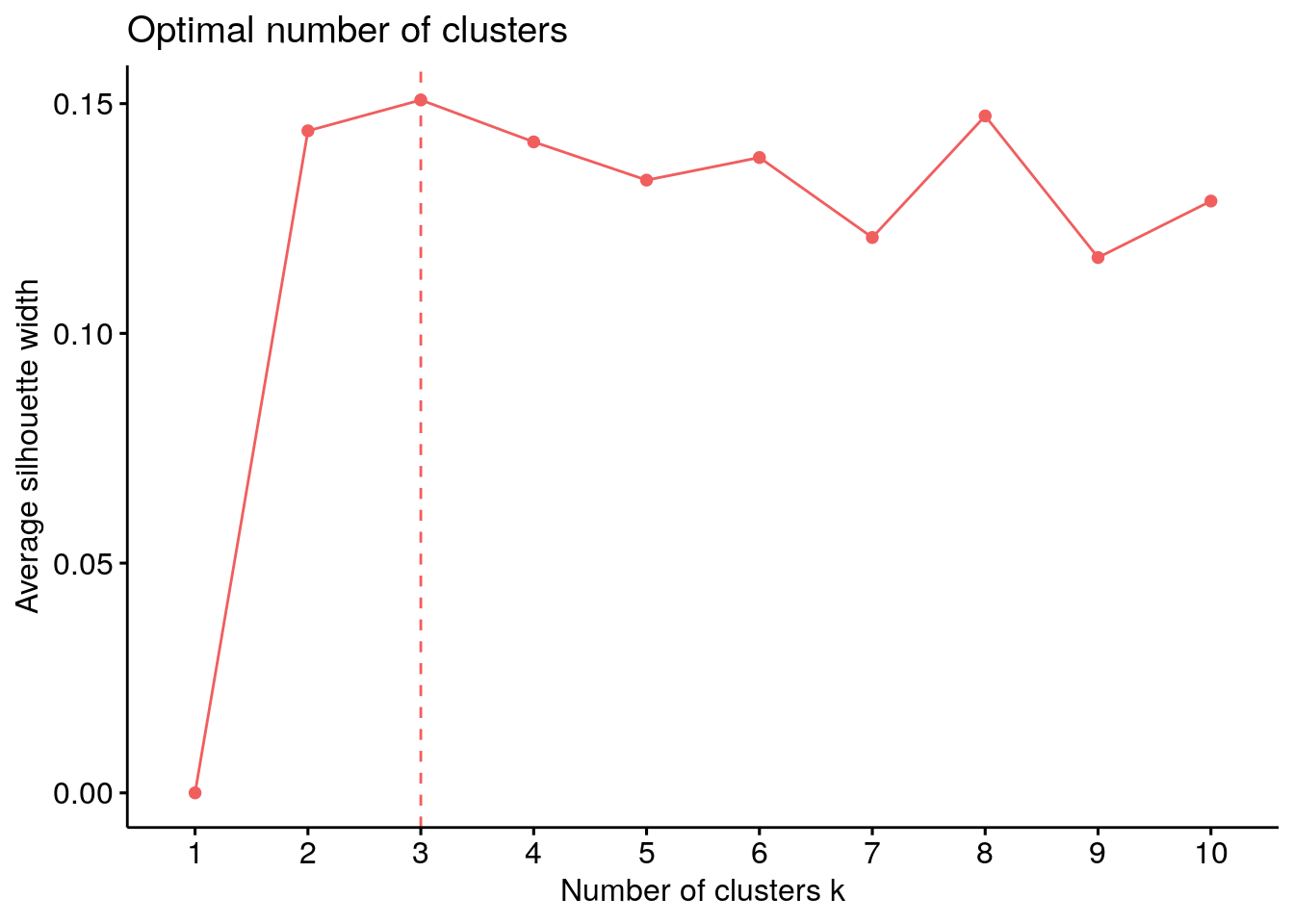
Figure 5: Optimal number of clusters when re-clustering the sprinters from step 1 using the silhouette appraoch.

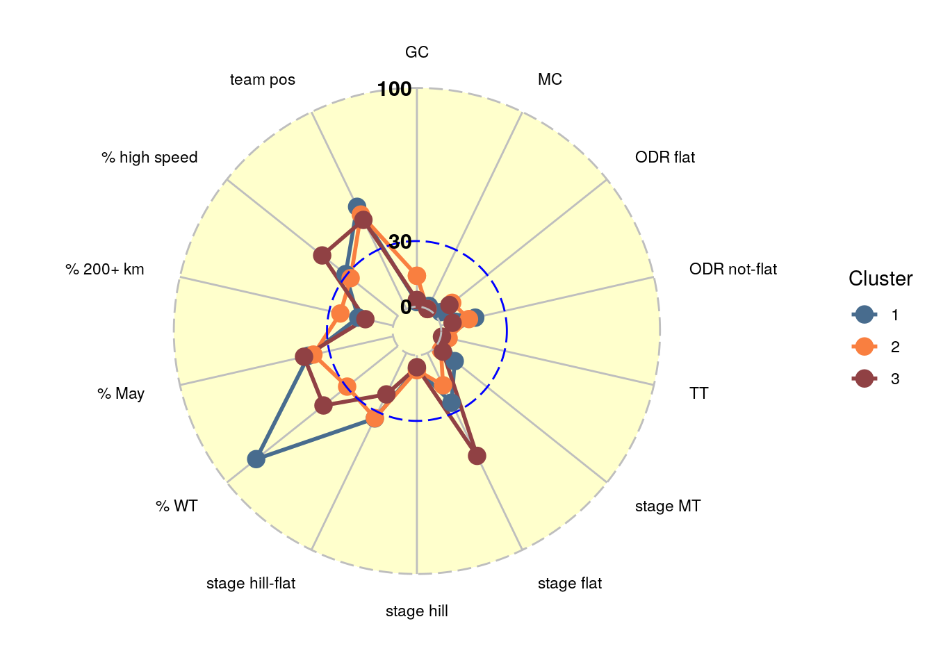
Figure 6: Scores per dimension for each second-stage sprint cluster in a radial plot.

The three sprint clusters show quite some variation in the new variables, in particular % WT and % high speed. It is not that straightforward to describe each cluster in just a few words, but we have tried our best. Cluster 3.1 can be characterized as all-round sprinters and classics riders at the world tour level, cluster 3.2 are the sprinters that score some GC points and love races of 200 kilometers or more. Finally cluster 3.3 is occupied by the pure strength, high-speed flat stage guys. The five most characteristic riders and riders with most points in each cluster are listed below.

cluster 3.3: High speed / super flat (40 riders)

• most characteristic: Giacomo Nizzolo, Dylan Groenewegen, Álvaro José Hodeg, Kristoffer Halvorsen, Luka Mezgec
• top scoring: Alexander Kristoff, Arnaud Démare, Dylan Groenewegen, Pascal Ackermann, Marc Sarreau

Finally, lets zoom in on the all-round sprint cluster 3.1. In Figure 7 we plotted the scores of the most characteristic riders in cluster 3.1, whereas in Figure 8 you can find the best scoring riders in this cluster. From the most characteristic riders in this cluster Sacha Modolo stands out on the hill-flat stages, and Mike Teunissen is in this cluster relatively strong on the GC dimension. When we look at the riders with most points we notice that Peter Sagan collects all his points from World Tour races. This is consistent with our extensive analysis of Sagan’s historic results.

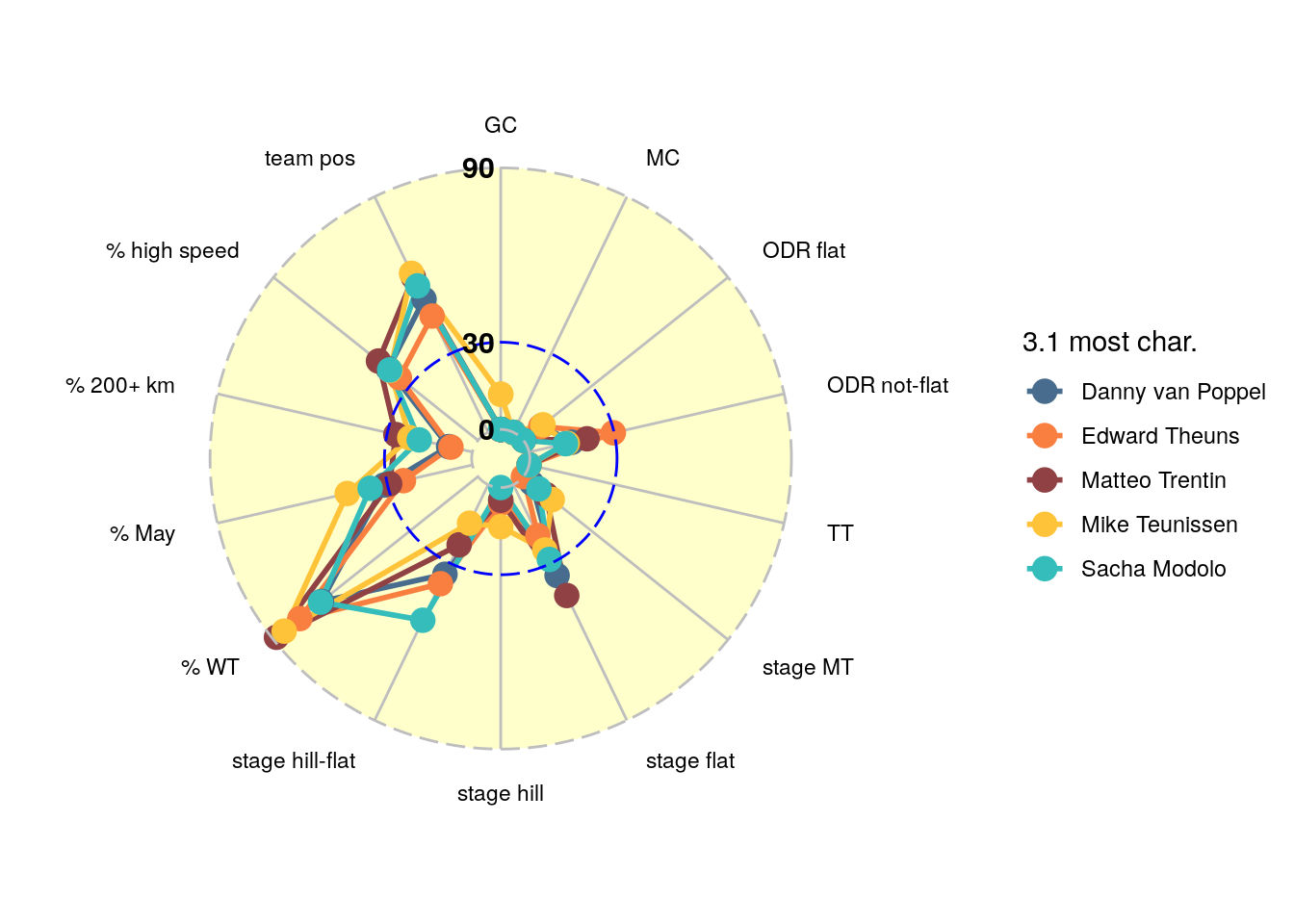
Figure 7: Scores per dimension for the most characteristic all round spinters in cluster 3.1

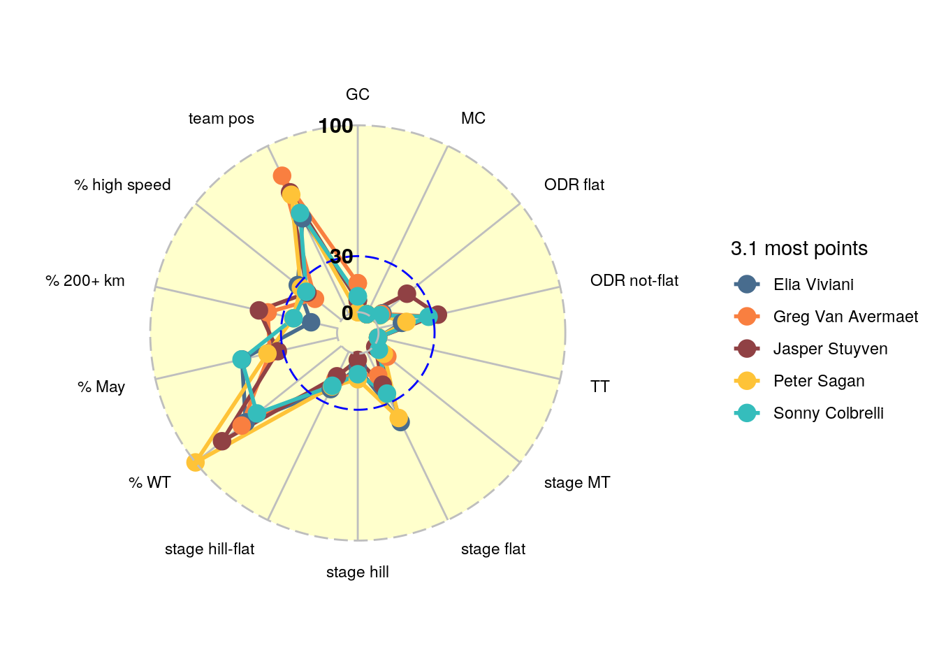
Figure 8: Scores per dimension for the best scoring all round spinters in cluster 3.1

Conclusion

The two-step approach when clustering riders is a considerable improvement over the single step approach that we tried earlier. The first step yields four clearly defined clusters consisting of time trialists, sprinters, GC guys/climbers and classics specialists. In the second step we looked at sprinters. Within the sprinter cluster we obtained three subgroups: flat stage specialists, sprinters with a GC component that like long distances and World Tour level all-round/classics sprinters.

We will most likely follow up on this clustering post by investigating how these clusters members are distributed over the teams. If you have other suggestions don’t hesitate to send us a message on Twitter or email.